NeRF was an Oral presentation at ECCV 2020 and had a significant impact, essentially creating a new approach from the ground up for scene reconstruction based on neural network implicit representations. Due to its simple concept and excellent results, many 3D-related works are still based on it today.
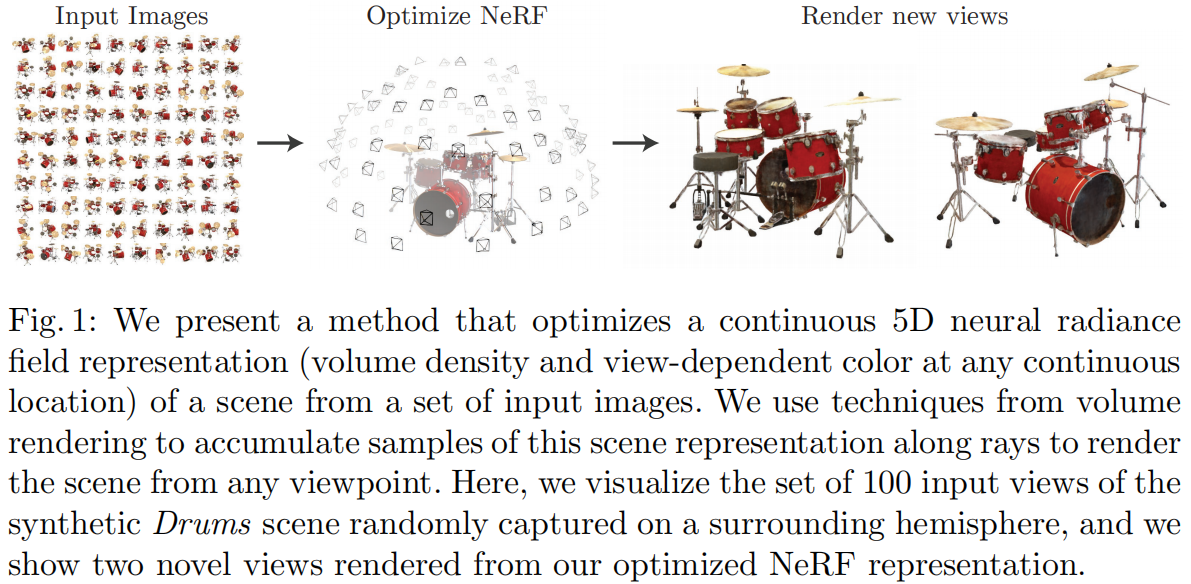
The task NeRF performs is Novel View Synthesis, which involves observing a scene from several known viewpoints (camera intrinsics and extrinsics, images, poses, etc.) and synthesizing images from any new viewpoint. In traditional methods, this task is typically achieved by 3D reconstruction followed by rendering. NeRF aims to bypass explicit 3D reconstruction and directly render images from new viewpoints based on the camera parameters. To achieve this, NeRF uses a neural network as an implicit representation of a 3D scene, replacing traditional methods like point clouds, meshes, voxels, or TSDFs. This network can directly render projection images from any angle or position.

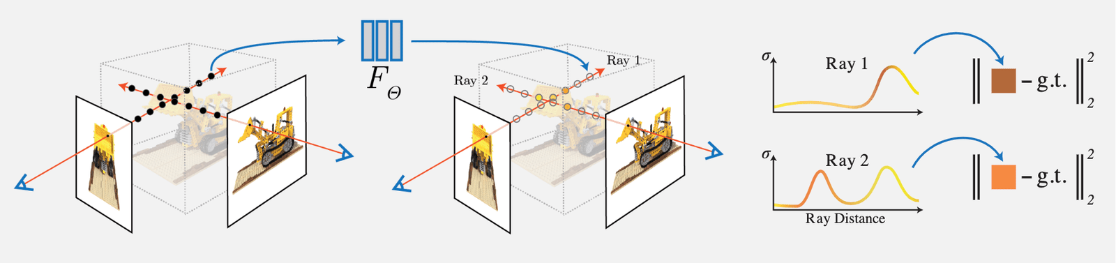
The concept of NeRF is relatively simple: it performs volumetric rendering by integrating the density (opacity) along the ray corresponding to each pixel in the input view, and then compares the rendered RGB value of that pixel with the ground truth as the loss. Since the volumetric rendering designed in the paper is fully differentiable, the network can be trained:

The main contributions and innovations are as follows:
1) Proposing a method to represent complex geometry + material continuous scenes using a 5D Neural Radiance Field, parameterized by an MLP network.
2) Proposing an improved differentiable rendering method based on classical Volume Rendering, which can generate RGB images through differentiable rendering and use them as optimization targets. This part includes an acceleration strategy using hierarchical sampling to allocate the MLP's capacity to visible content areas.
3) Proposing a Position Encoding method to map each 5D coordinate to a higher-dimensional space, allowing the neural radiance field to better express high-frequency details.

1 Neural Radiance Field Scene Representation

NeRF represents a continuous scene as a 5D vector-valued function, where:

• Input: 3D position \mathbf{x}=(x, y, z) and 2D viewing direction (\theta, \phi)
• Output: Emitted color \mathbf{c}=(r, g, b) and volumetric density (opacity) \sigma.

The 2D viewing direction can be intuitively explained by the following diagram:

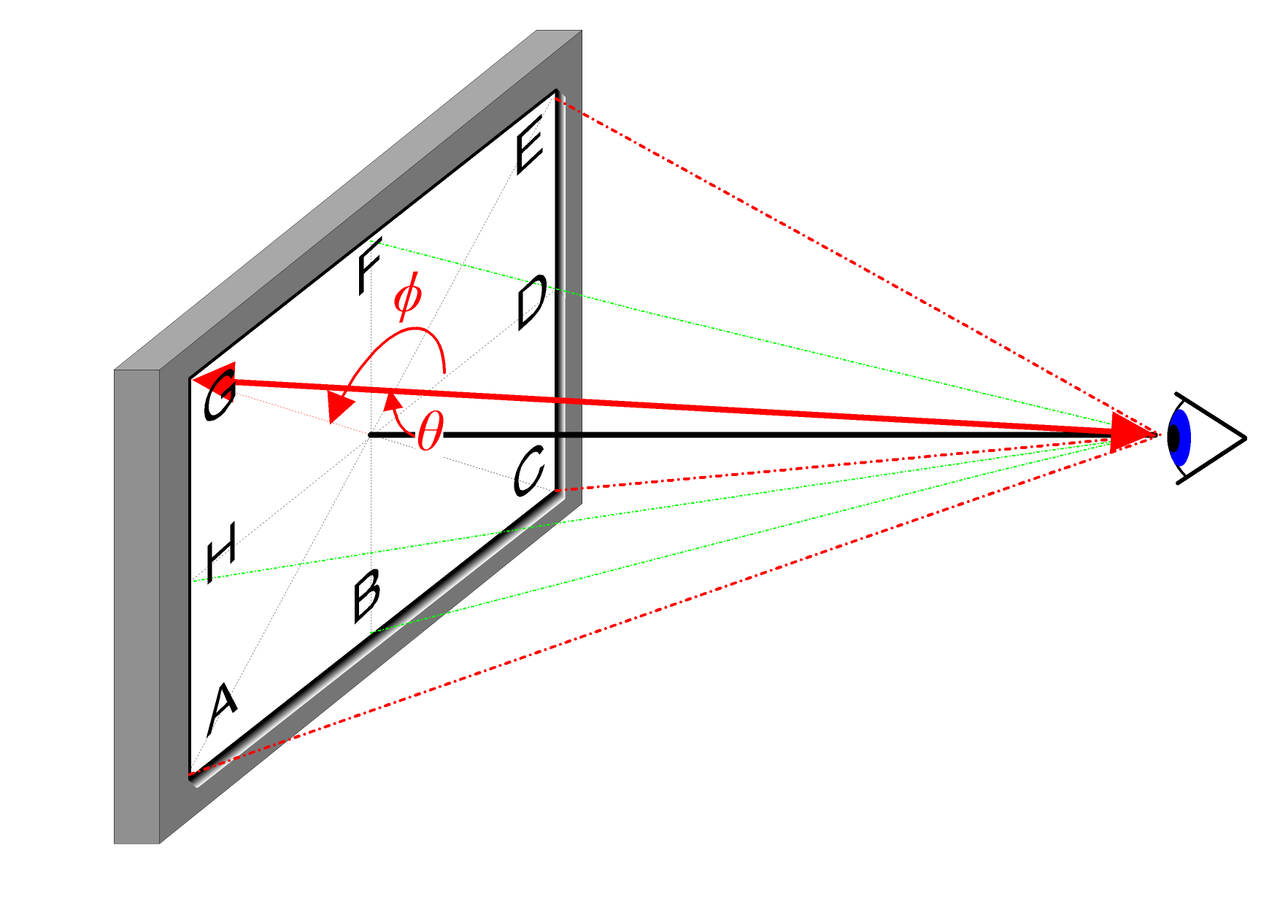
In practice, the viewing direction is represented as a unit vector in a 3D Cartesian coordinate system \mathbf{d}, which is the line connecting any point in the image to the camera's optical center. We use an MLP fully connected network to represent this mapping:
\begin{equation}F_{\Theta}:(\mathbf{x}, \mathbf{d}) \rightarrow(\mathbf{c}, \sigma)\end{equation}

By optimizing the parameters \Theta of this network, we learn the mapping from a 5D coordinate input to the corresponding color and density output.

To enable the network to learn multi-view representations, we make the following two reasonable assumptions:

• Volumetric density (opacity) \sigma is only related to the 3D position \mathbf{x} and is independent of the viewing direction \mathbf{d}. The density of an object at different positions should be independent of the viewing angle, which is quite obvious.
• Color \mathbf{c} is related to both the 3D position \mathbf{x} and the viewing direction \mathbf{d}.

The part of the network predicting volumetric density \sigma only takes the position \mathbf{x} as input, while the part predicting color \mathbf{c} takes both the viewing direction and position \mathbf{d} as input. In the specific implementation:

• The MLP network F_{\Theta} first processes the 3D coordinates \mathbf{x} with 8 fully connected layers (using ReLU activation, each layer with 256 channels) to obtain \sigma and a 256-dimensional feature vector.
• This 256-dimensional feature vector is concatenated with the viewing direction \mathbf{d} and fed into another fully connected layer (using ReLU activation, each layer with 128 channels) to output the RGB color related to the direction.

A schematic of the network structure used in this paper is as follows:

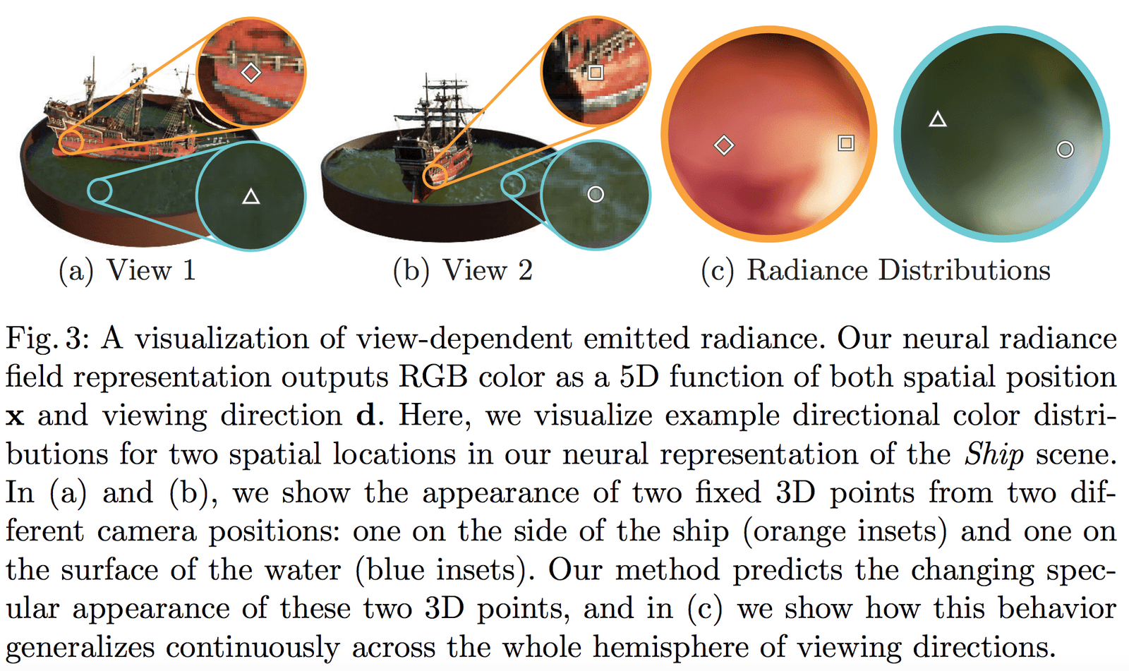
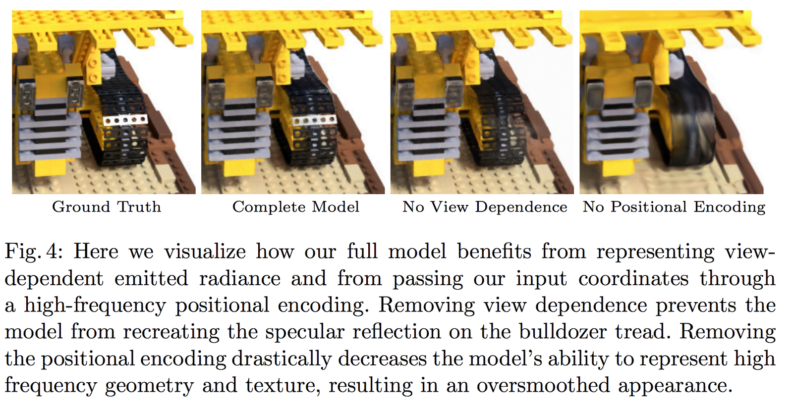
Figure 3 shows that our network can represent non-Lambertian effects; Figure 4 shows that if the input does not include view dependence (only \mathbf{x}), the network cannot represent specular highlights.

2 Volume Rendering with Radiance Fields

2.1 Classical Rendering Equation

To understand the concepts of Volume Rendering and Radiance Fields in the paper, let's first review the most fundamental rendering equation in computer graphics:
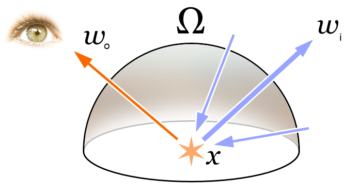
\begin{equation}\begin{array}{l}L_{o}(\boldsymbol{x}, \boldsymbol{d}) &=L_{e}(\boldsymbol{x}, \boldsymbol{d})+\int_{\Omega} f_{r}\left(\boldsymbol{x}, \boldsymbol{d}, \boldsymbol{\omega}_{i}\right) L_{i}\left(\boldsymbol{x}, \boldsymbol{\omega}_{i}\right) \left(\boldsymbol{\omega}_{i}, \boldsymbol{n}\right) d \boldsymbol{\omega}_{i}\\&=L_{e}(\boldsymbol{x}, \boldsymbol{d})+\int_{\Omega} f_{r}\left(\boldsymbol{x}, \boldsymbol{d}, \boldsymbol{\omega}_{i}\right) L_{i}\left(\boldsymbol{x}, \boldsymbol{\omega}_{i}\right) \cos \theta d \boldsymbol{\omega}_{i}\end{array}\end{equation}

As shown in the figure above, the rendering equation expresses the radiance (outgoing light) L_{o}(\boldsymbol{x}, \boldsymbol{d}) at a 3D spatial position \mathbf{x} in direction \mathbf{d}. This radiance is the sum of the emitted radiance L_{e}(\boldsymbol{x}, \boldsymbol{d}) from the point itself and the reflected radiance from external sources. Specifically:

• L_{e}(\boldsymbol{x}, \boldsymbol{d}) represents the radiance emitted from \mathbf{x} in direction \mathbf{d} as a light source.
• \int_{\Omega} f_{r}\left(\boldsymbol{x}, \boldsymbol{d}, \boldsymbol{\omega}_{i}\right) L_{i}\left(\boldsymbol{x}, \boldsymbol{\omega}_{i}\right) \cos \theta d \boldsymbol{\omega}_{i} represents the integral over the hemisphere of incoming directions.
• f_{r}\left(\boldsymbol{x}, \boldsymbol{d}, \boldsymbol{\omega}_{i}\right) is the scattering function, representing the proportion of radiance reflected from the incoming direction to the outgoing direction at this point.
• L_{i}\left(\boldsymbol{x}, \boldsymbol{\omega}_{i}\right) is the radiance received from direction \boldsymbol{\omega}_{i}.
• \boldsymbol{n} is the normal at 3D spatial position \mathbf{x}, and \theta is the angle between \boldsymbol{\omega}_{i} and \boldsymbol{n}, with \left(\boldsymbol{\omega}_{i}, \boldsymbol{n}\right)=\cos \theta.

To simplify the concept of radiance, in physics, light is electromagnetic radiation. We know the relationship between the wavelength \lambda and frequency \nu of electromagnetic waves is:
\begin{equation}c=\lambda \nu\end{equation}

That is, their product equals the speed of light c. We also know that the color RGB of visible light is the result of different frequencies of light radiation acting on the camera. Therefore, in NeRF, the radiance field is considered an approximation model for color.

2.2 Classical Volume Rendering Method

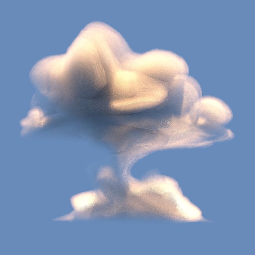
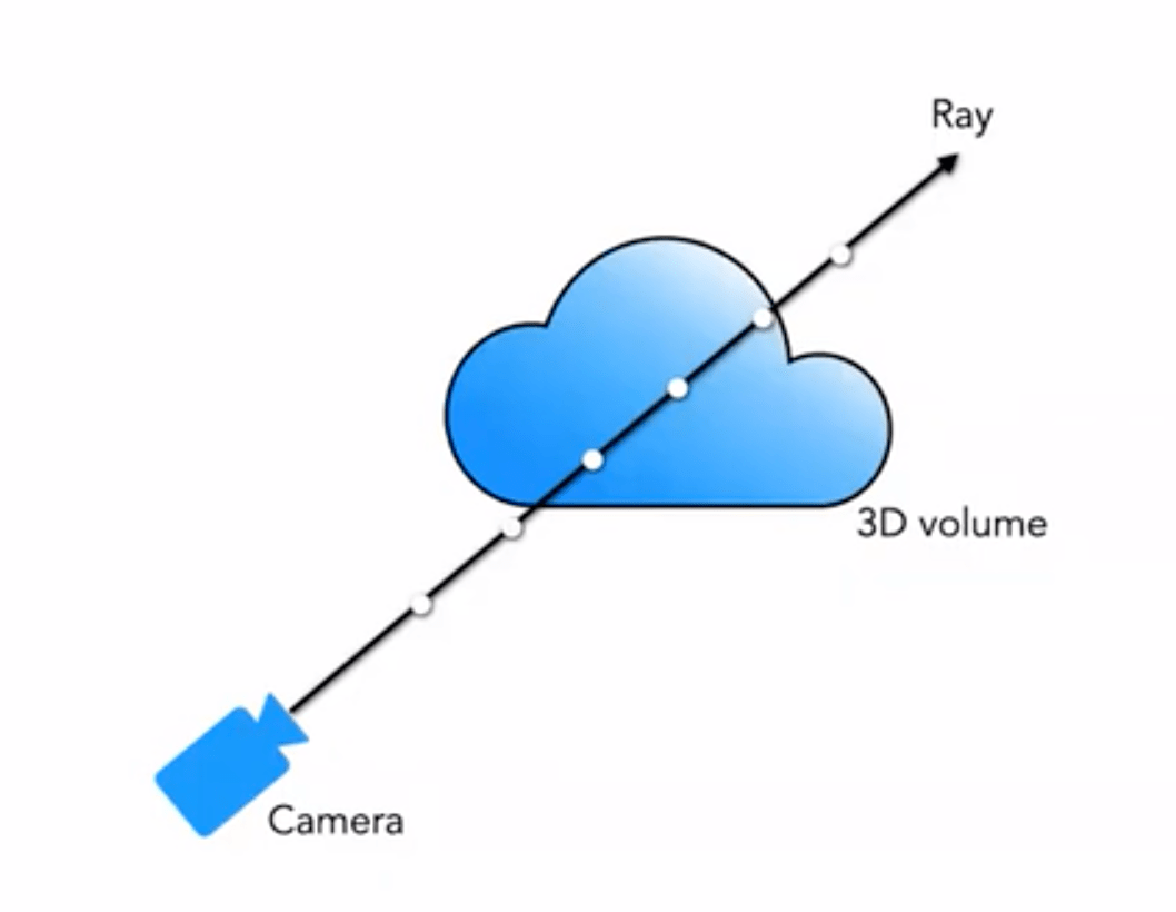
We are often familiar with rendering methods such as mesh rendering and volume rendering. For many effects like clouds, smoke, etc., volume rendering is commonly used:

Our 5D neural radiance field represents the scene as the volumetric density and directional radiance at any point in space. The volumetric density \sigma(\mathbf{x}) is defined as the differential probability of a ray terminating at an infinitesimal particle at position \mathbf{x} (or it can be understood as the probability of a ray stopping after passing through this point). Using the principles of classical volumetric rendering, we can render the color of any ray passing through the scene.

For a ray originating from viewpoint \mathbf{o} in direction \mathbf{d}, the point it reaches at time t is:
\begin{equation}\mathbf{r}(t)=\mathbf{o}+t \mathbf{d}\end{equation}
Then, by integrating the color along this direction over the range (t_n, t_f), we obtain the final color value C(\mathbf{r}):

The function T(t) represents the accumulated transmittance of the ray from t_n to t, which is the probability that the ray passes through without hitting any particles. According to this definition, the rendering of the view is expressed as the integral of C(\mathbf{r}), which is the color obtained by the virtual camera along each ray passing through each pixel.

The function \sigma(\mathbf{x}) (The volume density \sigma(\mathbf{x}) can be interpreted as the differential probability of a ray terminating at an infinitesimal particle at location \mathbf{x}.)

2.3 Piecewise Sampling Approximation for Volume Rendering

However, in practice, we cannot perform continuous integration. We use quadrature methods for numerical integration. By using stratified sampling to divide the range \left[t_{n}, t_{f}\right] into uniformly distributed small intervals, we perform uniform sampling in each interval. The division method is as follows:
\begin{equation}t_{i} \sim \mathcal{U}\left[t_{n}+\frac{i-1}{N}\left(t_{f}-t_{n}\right), t_{n}+\frac{i}{N}\left(t_{f}-t_{n}\right)\right]\end{equation}

For the sampled points, we use a discrete integration method:
\begin{equation}\hat{C}(\mathbf{r})=\sum_{i=1}^{N} T_{i}\left(1-\exp \left(-\sigma_{i} \delta_{i}\right)\right) \mathbf{c}_{i}, \text { where } T_{i}=\exp \left(-\sum_{j=1}^{i-1} \sigma_{j} \delta_{j}\right)\end{equation}
Where \delta_{i}=t_{i+1}-t_{i} is the distance between adjacent samples.

The following diagram vividly demonstrates the process of volume rendering:

3 Optimizing a Neural Radiance Field

The above method is the basic content of NeRF, but the results obtained based on this are not optimal, with issues such as insufficient detail and slow training speed. To further improve reconstruction accuracy and speed, we introduce the following two strategies:

• Positional Encoding: This strategy allows the MLP to better represent high-frequency information, resulting in richer details.
• Hierarchical Sampling Procedure: This strategy enables the training process to more efficiently sample high-frequency information.

3.1 Positional Encoding

Although neural networks can theoretically approximate any function, experiments have shown that using only an MLP to process the input (x, y, z, \theta, \phi) cannot fully represent the details. This is consistent with the conclusion proven by Rahaman et al. in their work ("On the spectral bias of neural networks. In: ICML (2018)"), which shows that neural networks tend to learn low-frequency functions. Their work also demonstrates that by mapping the input through high-frequency functions into a higher-dimensional space, we can better fit the high-frequency information in the data.

Applying these findings to the task of neural network scene representation, we modify F_{\Theta} into a composition of two functions: F_{\Theta}=F_{\Theta}^{\prime} \circ \gamma, which significantly improves the performance of detail representation. Specifically:

• \gamma represents the encoding function that maps from \mathbb{R} to a higher-dimensional space \mathbb{R}^{2 L}.
• F_{\Theta}^{\prime} is the standard MLP network.

The encoding function used in this paper is as follows:

The function \gamma(\cdot) is applied to the 3D position coordinates \mathbf{x} (normalized to [-1, 1]) and the 3D viewing direction Cartesian coordinates \mathbf{d}. In this paper, we set L=10 for \gamma(\mathbf{x}); and L=4 for \gamma(\mathbf{d}).

Thus, the encoding length for the 3D position coordinates is: 3 \times 2 \times 10 = 60, and the encoding for the 3D viewing direction is 3 \times 2 \times 4 = 24, corresponding to the input dimensions in the network structure diagram.

Similarly, in Transformer, there is also a positional encoding operation, but it is fundamentally different from the one in this paper. In Transformer, positional encoding is used to represent the sequence information of the input, while here, positional encoding is used to map the input to a higher dimension, allowing the network to better learn high-frequency information.

3.2 Hierarchical Sampling Procedure

The hierarchical sampling procedure is derived from acceleration work in classical rendering algorithms. In the aforementioned volume rendering method, how points are sampled along the ray affects the final efficiency. If too many points are sampled, the computational efficiency is too low; if too few points are sampled, it cannot approximate well. A very natural idea is to sample densely near points that contribute significantly to the color and sparsely near points that contribute little. Based on this idea, NeRF naturally proposes a coarse-to-fine hierarchical sampling scheme.

Coarse part: First, for the coarse network, we sample N_c sparse points (c stands for Coarse) and modify equation (3) into a new form (adding weights):
\begin{equation}\hat{C}_{c}(\mathbf{r})=\sum_{i=1}^{N_{c}} w_{i} c_{i}, \quad w_{i}=T_{i}\left(1-\exp \left(-\sigma_{i} \delta_{i}\right)\right)\end{equation}
where the weights need to be normalized:
\begin{equation}\hat{w}_{i}=\frac{w_{i}}{\sum_{j=1}^{N_{c}} w_{j}}\end{equation}

Here, the weights \hat{w}_{i} can be regarded as a piecewise-constant probability density function (PDF) along the ray. Through this probability density function, the distribution of objects along the ray can be roughly obtained.

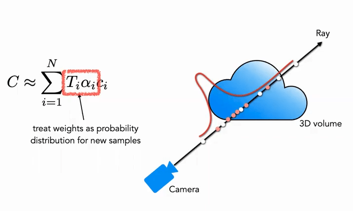
Fine part: In the second stage, we use inverse transform sampling to sample a second set N_f based on the above distribution. Finally, we still use equation (3) to compute \hat{C}_{f}(\mathbf{r}). The difference is that we use all N_c + N_f samples. Using this method, the second sampling can sample more points in regions with actual scene content based on the distribution, achieving importance sampling.

As shown in the figure, the white points are the points sampled uniformly in the first pass. After obtaining the distribution through the white uniform sampling, the second pass samples red points based on the distribution, with dense sampling in areas of high probability and sparse sampling in areas of low probability (similar to particle filtering).

3.3 Implementation Details

Regarding the training loss function, the definition in this paper is very simple and straightforward: both the coarse and fine networks use the rendered L_2 Loss, as shown in the following formula:
\begin{equation}\mathcal{L}=\sum_{\mathbf{r} \in \mathcal{R}}\left[\left\|\hat{C}_{c}(\mathbf{r})-C(\mathbf{r})\right\|_{2}^{2}+\left\|\hat{C}_{f}(\mathbf{r})-C(\mathbf{r})\right\|_{2}^{2}\right]\end{equation}

Where:

• \mathcal{R} represents the set of all sampled rays in a batch
• C(\mathbf{r}) represents the ground truth RGB color
• \hat{C}_{c}(\mathbf{r}) represents the RGB color predicted by the Coarse network
• \hat{C}_{f}(\mathbf{r}) represents the RGB color predicted by the Fine network

4 Results

This paper compares many related works such as:

• Neural Volumes (NV): https://github.com/facebookresearch/neuralvolumes
• Scene Representation Networks (SRN): https://github.com/vsitzmann/scene-representation-networks
• Local Light Field Fusion (LLFF): https://github.com/Fyusion/LLFF

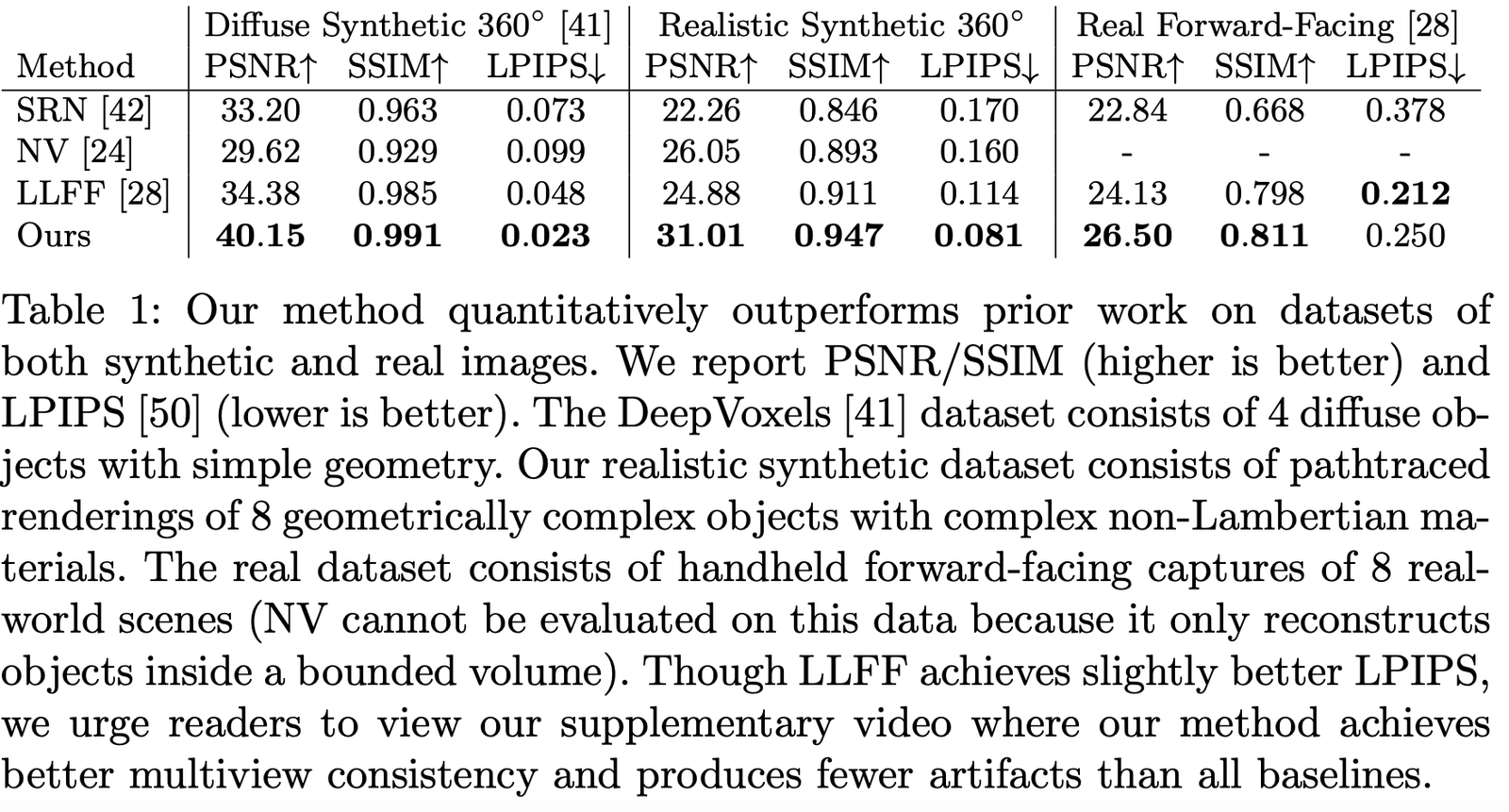
4.1 Datasets

The authors compared the performance on different datasets, and it can be seen that they are far ahead on almost all datasets:

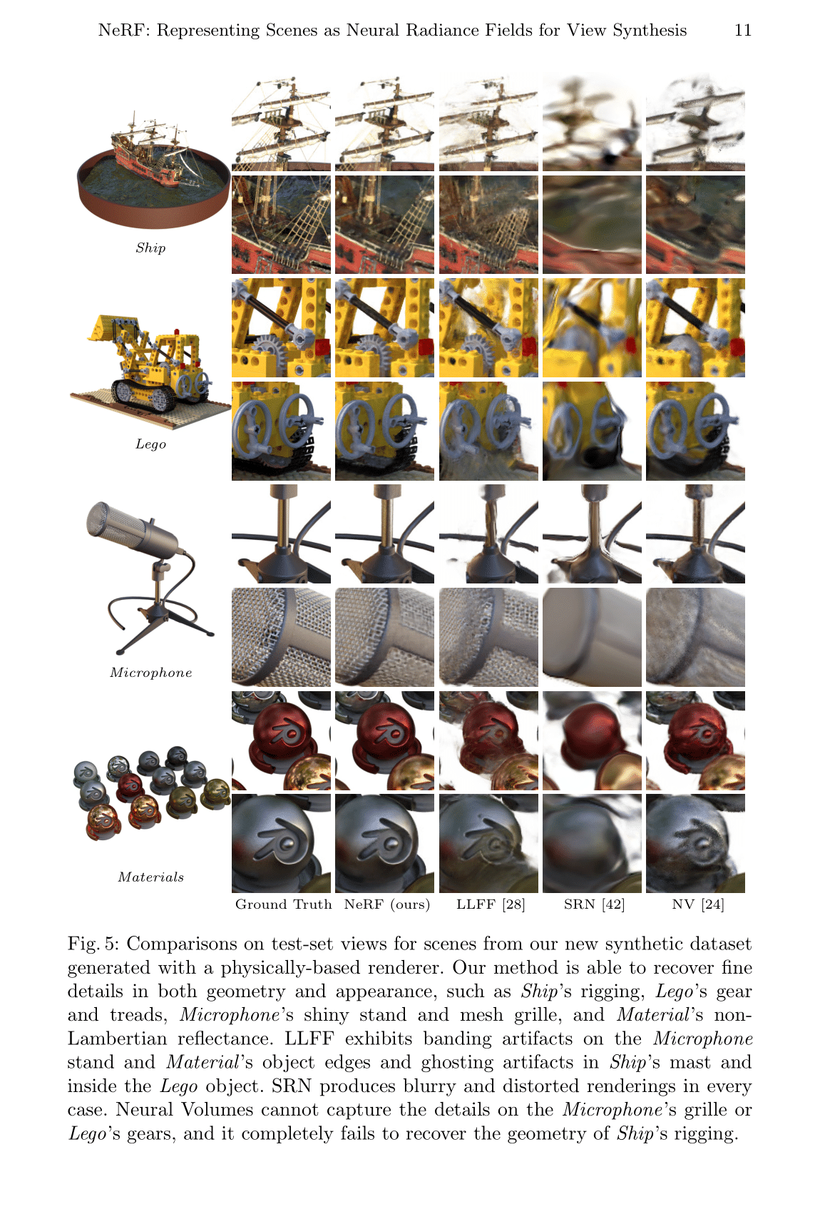
Visualization results on simulated datasets:

Visualization results on real datasets:

4.2 Ablation Studies

We conducted ablation studies with different parameters and settings on the Realistic Synthetic 360◦ dataset, with the results as follows:

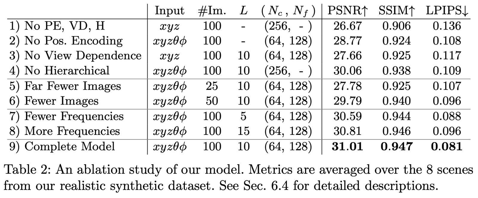
The main comparisons are as follows:

• Positional encoding (PE), i.e., \mathbf{x}
• View Dependence (VD), i.e., \mathbf{d}
• Hierarchical sampling (H)

Where:
The first row represents the smallest network without any of the above components;
Rows 2-4 represent removing one component at a time;
Rows 5-6 represent the effect of fewer sample images;
Rows 7-8 represent the effect of different frequency L settings (i.e., the frequency expansion level of positional encoding \mathbf{x}).

Paper Summary

The biggest innovation of this paper is bypassing the method of manually designing 3D scene representations through implicit expressions, allowing the learning of 3D information from higher dimensions. However, the downside is that it is very slow, which has been improved in many subsequent works. On the other hand, the interpretability and capability of implicit expressions still require more work to explore.
But in the end, it is believed that this simple and effective method will become a revolutionary point in 3D and 4D scene reconstruction in the future, bringing new breakthroughs to 3D vision.

Download Paper

PDF | Website | Code (Official) | Code (Pytorch Lightning) | Recording | Recording (Bilibili)
Colab Example: Tiny NeRF | Full NeRF

References

[1] Mildenhall B, Srinivasan P P, Tancik M, et al. Nerf: Representing scenes as neural radiance fields for view synthesis[C]//European Conference on Computer Vision. Springer, Cham, 2020: 405-421.
[2] https://www.cnblogs.com/noluye/p/14547115.html
[3] https://www.cnblogs.com/noluye/p/14718570.html
[4] https://github.com/yenchenlin/awesome-NeRF
[5] https://zhuanlan.zhihu.com/p/360365941
[6] https://zhuanlan.zhihu.com/p/380015071
[7] https://blog.csdn.net/ftimes/article/details/105890744
[8] https://zhuanlan.zhihu.com/p/384946242
[9] https://zhuanlan.zhihu.com/p/386127288
[10] https://blog.csdn.net/g11d111/article/details/118959540
[11] https://www.bilibili.com/video/BV1fL4y1T7Ag
[12] https://zh.wikipedia.org/wiki/%E6%B8%B2%E6%9F%93%E6%96%B9%E7%A8%8B
[13] https://zhuanlan.zhihu.com/p/380015071
[14] https://blog.csdn.net/soaring_casia/article/details/117664146
[15] https://www.youtube.com/watch?v=Al6NTbgka1o
[16] https://github.com/matajoh/fourier_feature_nets

Related Work

DSNeRF: https://github.com/dunbar12138/DSNeRF (SfM accelerated NerF)
BARF: https://github.com/chenhsuanlin/bundle-adjusting-NeRF
PlenOctrees: https://alexyu.net/plenoctrees/ (Using PlenOctrees to accelerate NeRF rendering)
https://github.com/google-research/google-research/tree/master/jaxnerf (Using JAX to speed up training)