This article combines traditional PnP methods with deep learning, with a relatively simple overall idea. The main focus is on how to backpropagate the residuals of the traditional PnP method to the neural network, enabling End2End training and computation without given data associations (Blind PnP).

1 Backpropagating a PnP solver (BPnP)

First, we describe the PnP problem using mathematical language.

Define g as a PnP solver, and its output y is the solved 6DoF pose:

Where x represents the 2D coordinate observations of feature points on the image, z represents the 3D point coordinates in space, representing a one-to-one mapping pair, and K is the camera intrinsic parameters:

begin{array}{l}boldsymbol{x}=left[begin{array}{llll}boldsymbol{x}_{1}^{T} & boldsymbol{x}_{2}^{T} & ldots & boldsymbol{x}_{n}^{T}end{array}right]^{T} in mathbb{R}^{2 n times 1} \boldsymbol{z}=left[begin{array}{llll}boldsymbol{z}_{1}^{T} & boldsymbol{z}_{2}^{T} & ldots & boldsymbol{z}_{n}^{T}end{array}right]^{T} in mathbb{R}^{3 n times 1}end{array}tag{2}
In fact, solving PnP is such an optimization problem:

boldsymbol{y}=underset{boldsymbol{y} in S E(3)}{arg min } sum_{i=1}^{n}left|boldsymbol{r}_{i}right|_{2}^{2}tag{3}
Where boldsymbol{pi}_{i}=pileft(boldsymbol{z}_{i} mid boldsymbol{y}, mathbf{K}right) is the projection function, and boldsymbol{r}_{i}=boldsymbol{x}_{i}-boldsymbol{pi}_{i} is the reprojection error.

Thus, we can simplify it as:

boldsymbol{y}=underset{boldsymbol{y} in S E(3)}{arg min } quad|boldsymbol{x}-boldsymbol{pi}|_{2}^{2}tag{4}
Where:

1.1 Implicit function differentiation

1.2 Constructing the constraint function f

Define the objective function of PnP as:

o(boldsymbol{x}, boldsymbol{y}, boldsymbol{z}, mathbf{K})=sum_{i=1}^{n}left|boldsymbol{r}_{i}right|_{2}^{2}tag{6}
When the objective function reaches its minimum, we have:

left.frac{partial o(boldsymbol{x}, boldsymbol{y}, boldsymbol{z}, mathbf{K})}{partial boldsymbol{y}}right|_{boldsymbol{y}=g(boldsymbol{x}, boldsymbol{z}, mathbf{K})}=mathbf{0}tag{7}
We define it as:

f(boldsymbol{x}, boldsymbol{y}, boldsymbol{z}, mathbf{K})=left[f_{1}, ldots, f_{m}right]^{T}tag{8}
Where:

1.3 Forward and backward pass

We first rewrite the PnP function, introducing the initial pose y^{(0)} :

boldsymbol{y}=gleft(boldsymbol{x}, boldsymbol{z}, mathbf{K}, boldsymbol{y}^{(0)}right)tag{10}
According to the implicit function differentiation rule:

begin{aligned}frac{partial g}{partial boldsymbol{x}} &=-left[frac{partial f}{partial boldsymbol{y}}right]^{-1}left[frac{partial f}{partial boldsymbol{x}}right] \frac{partial g}{partial boldsymbol{z}} &=-left[frac{partial f}{partial boldsymbol{y}}right]^{-1}left[frac{partial f}{partial boldsymbol{z}}right] \frac{partial g}{partial mathbf{K}} &=-left[frac{partial f}{partial boldsymbol{y}}right]^{-1}left[frac{partial f}{partial mathbf{K}}right]end{aligned}tag{11}
For neural networks, we can obtain the gradient of the output nabla boldsymbol{y}, and the gradients for each input are:

1.4 Implementation notes

2 End-to-end learning with BPnP

2.1 Pose estimation

This section describes the process of estimating the pose y based on the observed keypoint coordinates x, given a known map z and camera intrinsic parameters K, as shown below:

The loss is described by the following formula:

An important gradient update in the above process is calculated as follows:

The figure below demonstrates the convergence process in two cases, where the first row is lambda = 1 and the second row is lambda = 0.

Figure 1 represents h(I; theta) = theta

Figure 2 represents a modified VGG11 network

From these two experiments, we can see that both can converge regardless of whether the regularization term is used, and when lambda = 1, both achieve better convergence results.

2.2 SfM with calibrated cameras

This section is

The loss is defined as follows:

lleft(left{boldsymbol{y}^{(j)}right}_{j=1}^{N}, boldsymbol{z}right)=sum_{j=1}^{N}left|boldsymbol{x}^{(j)}-pileft(boldsymbol{z}^{(j)} mid boldsymbol{y}^{(j)}, mathbf{K}right)right|_{2}^{2}tag{15}
The gradient derivation in the process is as follows:

frac{partial ell}{partial boldsymbol{theta}}=sum_{j=1}^{N}left(frac{partial l}{partial boldsymbol{z}^{(j)}} frac{partial boldsymbol{z}^{(j)}}{partial boldsymbol{theta}}+frac{partial l}{partial boldsymbol{y}^{(j)}} frac{partial boldsymbol{y}^{(j)}}{partial boldsymbol{z}^{(j)}} frac{partial boldsymbol{z}^{(j)}}{partial boldsymbol{theta}}right)tag{16}
The figure below demonstrates the convergence process of an SfM:

2.3 Camera calibration

The camera calibration process is as follows:

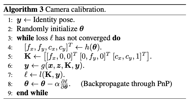
The loss is defined as follows:

l(mathbf{K}, boldsymbol{y})=|boldsymbol{x}-pi(boldsymbol{z} mid boldsymbol{y}, mathbf{K})|_{2}^{2}tag{17}
The gradient derivation is as follows:

3 Object pose estimation with BPnP

Finally, the author designed an object pose estimation process based on BPnP:

Paper & Code

Paper: https://arxiv.org/abs/1909.06043
Code: https://github.com/BoChenYS/BPnP
Video: https://www.youtube.com/watch?v=eYmoAAsiBEE